
First thing I noticed while writing this article is the red underline on convolutional – which really should not be there by now.
Convolutional Neural Networks (or CNN’s) are a type of neural network which utilises the concept of Convolution in order to process and analyse image data. The development of CNN’s in the area of deep learning accelerated and amplified the process of image analysis options far improving on the previous architecture of using an ANN to classify images. If you would like to read about ANN’s in depth check out my article on them here.
Convolution
Convolution is what we call an ‘Image Modifier’. It overlays a filter over parts of an image and detects patterns according to the filter (or ‘kernel’). This filter is a pattern finder which filters out everything unrelated to the pattern it is attempting to detect by multiplying irrelevant values or positions by 0 and adding higher correlation multiplication values or weights to certain positions which would warrant the detection of a pattern in that location or a feature of that particular pattern.
Convolutional can also be considered as a matrix multiplication; however, I will not be going in to depth on that as it is a redundant methodology as it takes up too much space in the system memory to be feasible for large images. This does however, introduce the idea of weight/parameter sharing which uses convolution in the place of an ANN’s weight matrix.
In the case of a coloured image the images gain a third colour dimension with RGB values.
Each neuron in a CNN represents a different filter which each look for a different feature within the images as aforementioned. These filters are vectorized in order to be processed by a computer.
Furthermore, since the outputs from the filters are 2-dimensional these outputs are stacked into a 3D form in order to be in the same shape as the input image (which when coloured has a 3rd dimension). These 2D outputs which are stacked are known as feature maps; aptly names as they represent the locations of the feature in an image.
The bias term is constant for each pixel and is not as relevant when looking at CNN’s as it mathematically is illegal but computes in code.
CNN’s use exponentially less weights for image processing than the original ANN architecture implementation due to the feature sharing methodology of CNN’s which is drawn from the concept of using the feature maps.
Another reason that ANN’s perform poorly at image classification in comparison to CNN’s is because they have to learn different weights for the same features depending on where in the image that feature is present whereas due to the concept of convolution and how a filter passes over the whole image, that is not required in a CNN.
Filters, and their weights, are found and modified through gradient descent as in all neural network architectures.
Architecture
Typical CNN’s contain a series of convolutional and pooling layers which then goes into a regular Dense ANN layer.
The pooling layer in a CNN downsizes images for the next convolutional layer based on either max or average pooling – which is a hyperparameter choice. Max pooling takes sample squares and returns the max value and average pooling does the same with the average value instead. This shrinks the image and means that less data needs to be processed, and allows for Translational Invariance which means that it does not matter where in the image the feature is present – just that the feature itself is present and tells the network whether the pattern was found or not without needing to store the location and positions of where the pattern was found.
The filter size stays the same after pooling even though the image shrinks which allows each additional layer of a CNN to look at larger and more complex features of an image dataset which allows CNN’s to learn hierarchical features – how different features are combined to create larger and more specific and complex features.
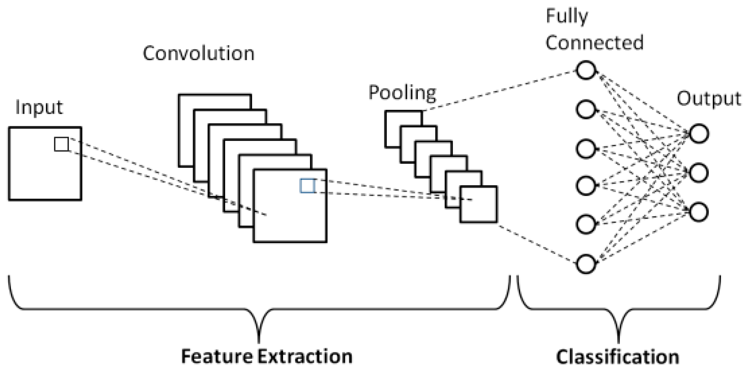
The Dense layer at the end of the network takes the flattened output of the previous layers and uses regular classification techniques in order to classify the image into different categories based on the output from the convolutional and pooling layer series. The regular softmax function is used in order to compute the final classification prediction and the sparse categorical cross entropy loss function computes the loss for the network to allow gradient descent to modify the weights and biases of the dense, convolutional, and pooling layers of the entire network.
I was not able to go into very much depth into the CNN mathematics since I am pressed for time studying for exams so I hope I can be forgiven. Perhaps some time in the future I will revisit this topic when I have enough time and offload the equations onto the blog. Thank you for reading and I really hope you are enjoying my blog.
