Gradient Descent, Optimizers, and How a Neural Network ‘Learns’

To start off, all three of the above are the same. A Neural Network ‘learns’ by means of its optimizer, and all optimizers are versions of and different implementations of Gradient Descent.

But what is Gradient Descent?

To understand Gradient Descent, let’s look first look at a Neural Network. When a network makes a prediction, it compares this prediction against the actual value, to see how wrong it is. This measure of incorrectness is computed through the loss function of the network. Loss functions are also known as cost functions and error functions.

An example of a loss function is Mean Squared Error. This function takes the difference between the predicted value and the actual value and squares it. It takes the sum of all of these squared differences and divides it by the number of predictions to get the mean of the squared error.

Where N is the number of predictions made which is the same as the number of data samples

Now the prediction_i made by a network is a combination of its various input features, their weights, and the bias all passed through the activation function. If you would like to understand this article better, please go back and read my articles on Artificial Neurons, and Artificial Neural Networks.

All of these weights and biases are randomly initialised, and are therefore not tuned to be accurate. The goal of the network is to have as small of a loss as possible, and therefore have the highest possible accuracy. To do this we would need to find the point on the loss function where the resultant loss is as small as possible, aka the minima of the loss function.

https://theneuralnetworkblog.wordpress.com/wp-content/uploads/2020/06/3285b-1melyetzstijrnnki8ktkcw.jpeg

If you know basic calculus, when there is a function (say f(x)), to find the minimum we differentiate the function and equate the derivative to 0. However, for the loss function we have more than one input. We have all the weights and biases of the network which are used to calculate the predicted value.

In this case we need to use Multi-Variable calculus. This methodology uses partial derivatives in order to find the direction of steepest increase. If we take the negative and reverse that direction, we get the direction in which the loss function decreases the most – the direction of steepest decrease.

Based on the partial derivatives of the loss function relative to every parameter, we update and change each weight and bias by the learning rate multiplied by the value of this derivative. This modifies each weight and bias in the direction of lowering the loss function towards its minimum.

You should be wondering, what is this learning rate thing I speak of?

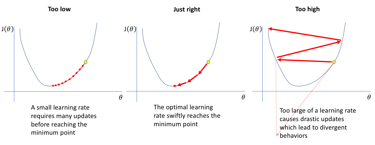
Well, the learning rate actually has a very apt name. It is the degree to which each weight and bias changes. This controls and ensures that the change applied to each parameter does not overshoot – which is when the parameter modification is so large but there is a small distance to the actual minimum, which results in the loss function missing that minimum and overshooting to the other side.

By multiplying the learning rate by the change applied, we can ensure that this does not happen. However, this is a hyperparameter meaning some parameter which affects the output of the network, but not directly, and cannot be trained. This is something the programmer has to choose themselves.

This is a very important decision to make. If the learning rate is too high then the network will overshoot the minimum of the loss function. If it is too low then the model will be sample-inneficient and will be very slow to learn. The correct value for the learning rate must be chosen through experimentation. A good learning rate prevents overshooting without sacrificing too much speed.

https://www.jeremyjordan.me/content/images/2018/02/Screen-Shot-2018-02-24-at-11.47.09-AM.png

When the loss function reaches a point where the parameters are not being updated and changed (when the gradients are equal or tending to 0) and therefore the loss is constant, the network has completed learning/optimizing. This does not mean that a network is 100% accurate though. It only means that the current network model and hyperparameters are as optimized and therefore as accurate as possible.

In order to increase accuracy at this time we must modify the hyperparameters and the model in order to change the loss function to a point where it has a minimum that is less than before.

Other Optimizers

Now Gradient Descent is the basic optimizer, the original concept on which more modern and improved optimizers are built. I will only go over them briefly here but if you would like to learn more, do drop a comment or contact me through the blog and I can clarify or write a more extensive article on them.

Stochastic/Batch Gradient Descent

As you may have guessed from the name, this deals with applying Gradient Descent in batches. The main purpose of SGD is to optimise computation as by taking a random selection of data from a large dataset in a batch should yield an approximate mean/range of values similar to the entire dataset. This means we have to load less data into memory and do significantly less computation as we don’t need to go through the whole dataset at once – instead going through it in batches.

These batches are shiffles and randomised (keeping correlations between inputs and outputs of course) to ensure that the network does not simply memorise connections and actually ‘learns’.

for epoch in range(0, epochs):
    inputs, outputs = shuffle(inputs, outputs)
    for i in range(size of dataset / batch size):
        start = i * batch size
        end = (i+1) * batch size
        inputBatch, outputBatch = inputs[start:end], outputs[start:end]
        *Gradient Descent on Batches*

Gradient Descent with Momentum

This implementation includes some ideas from physics. By applying a friction coefficient and creating a momentum effect on the change applied this implementation creates a sliding effect in the change, allowing each step to have a greater effect than initially. This speeds up training and finds a minimum faster than traditional gradient descent.

Without momentum the step taken by the algorithm could be inefficient for some parameters as their gradients might not be very steep meaning that they won’t change much. Once momentum is applied these smaller gradients accumulate and can have a bigger impact on the actual parameter, allowing bigger steps/changes to be made to a parameter with a small gradient. This speeds up learning by speeding up the training of so called ‘shallow’ gradient parameters.

Variable Learning Rates

This was devised as an alternative way to speed up and improve gradient descent as compared to momentum. What this does is it changes the learning rate of a network by a certain factor after a set number of timesteps or iterations (epochs). This could be linear (constant factor) or exponential (exponential factor). There is also proportional decay in which the learning rate decreases proportional to the time/iterations which have passed. The speed of all of these techniques can be modified by adjusting their factor values.

These were meant to prevent networks from overshooting by decreasing the learning rate the more the network learns, allowing it to take smaller step sizes as it got closer to the minimum. By doing this the network would only make smaller changes as it got nearer to the minimum of the loss function – eradicating the possibility of overshooting. A big issue with this approach was that it added more hyperparameters for the programmer to experiment with and choose values for.

Adaptive Learning Rates

These follow the philosophy that not every parameter of the network has the same impact/contribution to the loss. Some may contribute a lot and some may contribute a little and therefore each parameter requires its own adapting learning rate which is changed individually for that weight or bias.

First came AdaGrad which introduced the idea of having a cache which was the accumulation of the squared gradients of that parameter. This allowed the network to gauge how much each parameter has already learned, and therefore how much more learning it requires. The higher the cache value, the lower the learning rate.

This was done by dividing the learning rate times the gradient by the square root of the cache plus epsilon (a really small value which existed just to prevent dividing by 0) This made the parameter update function look like this:

However, AdaGrad was found to decrease the learning rate too quickly and it approached 0 much before learning was complete. RMSProp was introuduced to solve this issue. This approach decreased the existing cache before adding the new squared gradient. This was known as the decay. The update function was the same as AdaGrad’s but cache function for RMSProp looked like this:

The cache is usually initialised as 1 so that the first individual learning rate for each parameter is the same as the base general learning rate.

Finally came Adam. This is the current industry standard and the theory and mathematics behind it is way out of the scope of this article. To sum it up, Adam is known as RMSProp with Momentum. It combines the ideologies of RMSProp’s cache with Momentum’s ability to keep track of previous gradients using friction as well as some degree of bias correction in order to update and change parameters.

https://3qeqpr26caki16dnhd19sv6by6v-wpengine.netdna-ssl.com/wp-content/uploads/2018/11/Line-Plots-of-Train-and-Test-Accuracy-for-a-Suite-of-Adaptive-Learning-Rate-Methods-on-the-Blobs-Classification-Problem.png

---

Please keep in mind that Adaptive Learning Rate techniques are not necessarily the best. In some cases regular Gradient Descent performs better than them. Choosing an optimizer for a neural network is a hyperparameter chosen by the programmer and is dependent on the task and data that the neural network is being created to use.

I hope you enjoyed reading this article as much as I enjoyed writing it! Please leave some comments below with feedback, thoughts, and criticism on my writing – everything helps and I would love to know what you thought. My hope is that my writing is sharing my love for these topics with the world and perhaps inspiring some people to look into and explore Deep Learning and Artificial Intelligence. Thank you so much for reading!